Curious Similarities Between AI Architectures and the Brain

On the question of how close is the machinery of modern artificial intelligence to biological processes of reasoning we went through the whole spectrum during the last decade, jumping all the way from bold headlines like “A New Supercomputer Is the World’s Fastest Brain-Mimicking Machine“ and “A Supercomputer That Works Like The Human Brain Has Just Been Turned On“ down to realisations “Why Artificial Intelligence Will Never Compete With the Human Brain“, questions like “Do neural networks really work like neurons?“ and direct calls to action: “Stop comparing human intelligence and AI – they are completely different“. I am sure you have seen your share of headlines from both camps. As usual, after trying out the extremes, the public opinion has converged on a sensible balanced option in the middle, noted that “Neuroscience and artificial intelligence can help improve each other“, explained “How AI and neuroscience drive each other forwards“ and charted a path towards “Neuroscience-Inspired Artificial Intelligence“.

The reason why the bold claims on both the similarity and the dissimilarity could not hold, is simple — it is not possible to compare these two immensely complex systems in one headline, or even one article. To succeed and make the discussion fruitful we need a more granular and systematic approach.

In this piece I would like to apply a well-established method of analysis of complex systems (allowing for some freedom of interpretation), explore how it could help us organise the diversity of opinions on the topic at hand and see whether it can help us identify and leave some of the non-questions behind and bring to the light more interesting and important points and nuances we should be arguing about.

Table of Contents

• A way to structure the conversation
• Drastic differences at the level of implementation
• Curious similarities at the level of algorithms and representation
• Hippocampus, memory consolidation and experience replay
• Hierarchy of layers in visual systems
• Representing spatial information in grids
• Successor representations
• Predictive coding and GANs
• Visual attention
• Dopamine reward prediction and temporal difference learning
• Not only similarities: Backpropagation
• Conclusions about the level of algorithms and representations
• The common goal of computation

A way to structure the conversation

In 1976 David Marr and Tomaso Poggio proposed three levels at which a complex system could be analysed in order to be understood from the computational perspective (Marr and Poggio, 1976). The need for this mental framework arose from the question “at what level is it necessary and profitable to study the information processing that is carried out during visual perception?” (sic), which they then proceeded to explore in the context of machine vision vs. biological vision. For the purposes of our discussion, we extend the domain of application beyond the visual system, and replace “study” with “compare”. We now have a tool to apply to the question at hand: “at what level is it necessary and profitable to compare the information processing that is carried out by the human brain and an AI system?”.

According to Marr and Poggio the useful levels of analysis are: the computational level — the goal or theory of the computation, the level of algorithm and representation, and the level of implementation.

The level of implementation is the lowest level of abstraction where we compare the hardware / wetware components. By hardware in this case we broadly mean the physical system that carries out the computation, its basic components (transistors, neurons, synapses, electrical connections) and the physical phenomena (electricity, chemical reaction, mechanical interactions) that make those components work.

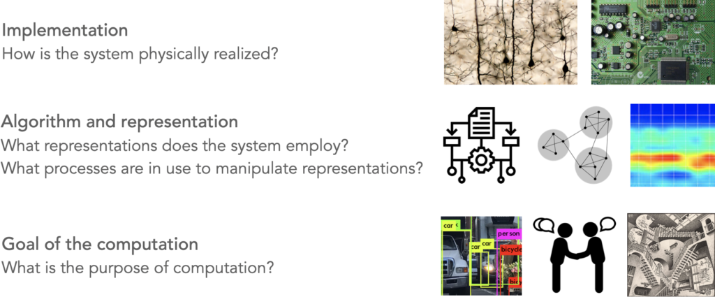
At the level of algorithm and representation we aim to compare data types and the structures that the system is using to store information and the computational methods it employs to manipulate that information. Examples of the data types could be: voltages, activation values, synaptic weights, oscillation powers, pixel intensities, etc. These, in turn, tend to be organised into structures: lists, matrices and tensors, graphs, trees, etc.

We can note here how operating at different levels of comparison already helps us in addressing the question of (dis)similarity of artificial and biological neural networks. We can see the similarities on the level of representation: both the artificial and biological networks have nodes (neurons, units) that are connected with each other (synapses, weights) forming a graph-like structure. But at the same time we see the differences at the level of implementation: artificial neurons are only simple and abstract models of their biological counterparts.

Once we have figured out what is the data we are working with and how it is stored we can proceed to the question of algorithms, that is — the methods of manipulating the data. Humans came up with a multitude of smart ways of solving various computational problems and called them algorithms. You probably have heard of such examples as Brute-force search, Dijkstra’s algorithm for finding a shortest path, Fourier Transform for decomposing a signal into its frequency components, Monte Carlo methods, and many others. A nice property of algorithms is that, by definition, they are unambiguous descriptions of how a particular computation or data manipulation should be carried out to achieve the desired result. What interests us in this discussion is which are the algorithms that our brain is using to solve the complex tasks we do every day: object recognition, navigation, logical reasoning, planning, sorting, etc. Can we find these algorithms, and by doing so obtain an unambiguous descriptions of how the brain functions? This is a fascinating question that the field of Computational Neuroscience is trying to answer by proposing various computational models and evaluating how likely it is that our brain is using one or another computational mechanism to solve a certain task. The latest revival of the notion of artificial neural networks being similar to mammalian brain arose from the observation that the artificial mechanisms that turned out to work well on certain tasks (such as visual object recognition) seem to share structural and algorithmic similarities with the mechanisms of our brain. And that led to the excitement.

The final level of comparison – the goal of computation – is the most abstract one. It concerns the reason why the computation is being carried out. What is the purpose of it. In the last section I will argue that since it is us, humans, who define the goals of AI systems, the purpose of those systems is frequently aligned with the goals of humans: generating text, finding best product options, identifying and categorising objects, recognising speech — all of these are the goals that are common between ourselves and the artificial systems we create. Having this category helps us distinguish between the questions of how and what and not mix them together in our discussion.

Now, once we have established the axes of comparison: implementation, representation & algorithm, and purpose, we can proceed to attempt the comparison.

Drastic differences at the level of implementation

The notion (and the associated hype) that the modern AI algorithms are brain-like came from the idea that on the most basic level the design principles of artificial neural networks are neuroinspired. Which is a word that does not tie you to any factual truths, but does catch the reader’s eye by referring to one of the greatest scientific puzzles of today — the human brain.

On the level of implementation (following Marr’s tri-level taxonomy we have established above), while there is a superficial similarity between biological neural networks and modern machine learning architectures, the specifics of engineering detail differ a lot. Let us take a closer look at the building blocks of artificial and biological networks — the neurons.

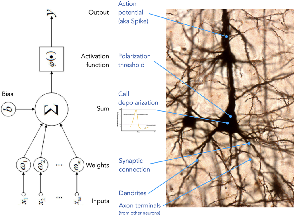
Frequently presented as an argument in favour of the similarities, an illustration like the one above can serve equally well as a list of differences:

topology and connectivity — In artificial neural networks we enjoy reliable, noiseless (unless we introduce the noise on purpose) and neatly organized connections between the layers of the networks. In a biological network the existence of a connection between a certain pair of neurons is not a guarantee, one cannot enjoy fully connected layers where each neuron from population A is guaranteed to be connected to each neuron in population B. Also random connections and influences that just formed because of how the tissue grew and not due to any grand design are present and active (which is not necessarily a limitation, such shortcuts might prove very useful).

synapses vs. weights — A synapse is a complex electrochemical system that facilitates the transmission of signal from from one (pre-synaptic) neuron to another (post-synaptic). There is a dedicated field of science, called molecular neuroscience, major part of which studies the different types of ion channels, different mechanisms of neurotransmitter release, properties of neurotransmitters and types of receptors that all together comprises the complex machinery that passes the signals in our nervous system. Meanwhile the artificial counterpart of a synaptic connection can be described here, in full, as follows: \(x_i * w_i\).

spike vs. output — In artificial neural networks (ANN) we have full control of the output of neuron’s activation function. In most cases it is a continuous value, within a fixed range (tanh, sigmoid) or unbounded (linear, ReLU). While in a biological network it is closer to a binary (with caveats we are not going to go into): a spike or no spike. As one can imagine this has enormous consequences on what kinds of computations can be carried out by artificial vs. biological “hardware”. Spiking Neural Networks (SNN) represent an attempt to make ANNs more biologically plausible, while they offer a significant reduction in power consumption, their computational capacity is much lower compared to regular ANNs and their use in practical application is limited. However they offer an interesting research platform for those believing that limiting ourself to the computational capabilities of human brain will put us in a better position to discover the mechanisms of it, as we will be only exploring those algorithms that are feasible on biological “hardware”.

polarization threshold vs. activation function — In addition to having a greater control over the output of an artificial neuron, we also have endless flexibility when deciding which condition should trigger that output. ReLU activation function, for example, allows to discard the values below 0 and only propagate the signal if the sum of inputs is positive. Tanh and Sigmoid allow to define the range of the output value. As long as the function is differentiable, we can define quite complex rules for how the input into the neuron should be transformed. Biological mechanism does not enjoy all that flexibility: action potentials arriving into a neuron cause the cell to depolarize, and, upon reaching neuron’s polarization threshold the neuron releases its action potential up the network.

timing — Signal propagation in an artificial neural network is happens synchronously along all of its connections and travels in cycles, even if a portion of the network will complete it’s computation slower, the rest will “wait” until all the necessary operation are completed before progressing to the next layer or cycle. The concept of time of arrival of a signal bears no importance and carries no role in the computations. This is opposite to how biological neural network operates. While there are certain synchronization mechanisms, largely signals are emitted and propagate very asynchronously and are affected by multitude of factors such as the length of a particular axon or dendrite, properties of the tissue in that particular region of the brain, type and structure of a cell, etc. The timing of when (and how often) a signal arrives plays a huge role and (just one example) serves as the key component for the mechanism of Spike-Timing-Dependent Plasticity, a process that controls the strength of connections between neurons, playing an essential role in learning and formation of a biological neural network. Timing is incorporated into the operating model of Spiking Neural Networks we mentioned above.

Many more such examples can be brought up, but the ones listed above are sufficient for the purpose of this conversation, and I believe, allow us say that at this lowest level of analysis we should side with the claim that apart from the superficial similarity between a biological neuron and an artificial neuron, the systems are fundamentally different.

Let us now see what we will discover on the next, more abstract, level of analysis.

Curious similarities at the level of algorithms and representation

As we move to a higher level of abstraction to the level of algorithms and representations, the design principles, representations and strategies of information processing in biological systems sometimes start to resemble the architectural principles that the best artificial systems rely on.

Hippocampus, memory consolidation and experience replay

Broadly speaking, there are three stages of memory storage and formation: first, an experience is stored in the working memory, and, unless there is a need, it will be there for a short number of seconds. If, however, this experience is deemed important or unusual by the brain, it gets to the second stage and becomes represented in the hippocampus. Here it can linger for hours or perhaps even days. The hippocampus is an interesting structure because it is connected to our cortical structures, acting, according to some theories, as a hub that connects different modalities that are represented in separate parts of the brain into one, binding visual, semantic, linguistic, sensory, motor and auditory aspects of an experience together. If that is the case it stands to reason that the flow of information also goes the other way — from the hippocampus to the cortex. This would happen when the brain decides to store an experience for good and is mediated by a process called consolidation, which sometimes requires repeated exposure to the same experience in order to get imprinted in our cortex.

This bears a curious similarity to one of the crucial components of early (and modern) deep reinforcement learning (DRL) system (Mnih, 2015) — a so-called replay buffer.

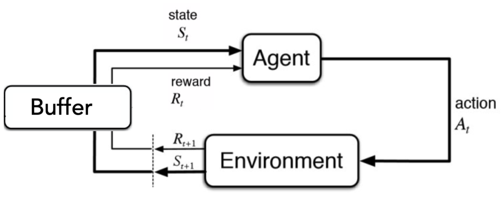
An agent (driven by a neural network) picks actions, carries them out in the environment, and observes how did the environment change as a result of that action and what, if any, was the reward (or penalty) for taking a particular action in a particular state. The initial state, the action, the reward and the next state form what is called a SARS tuple and in a way represent an experience. In off-policy DRL algorithms, these experiences are stored in a replay buffer. In addition to the experience-gathering loop there is another process running in parallel – the learning loop, during which the neural network (the one that decides which actions the agent should take) is being tuned to prefer and pick actions that lead to rewards. During learning the experiences from the replay buffer are sampled again and again and are, in a way of analogy with the biological process described above, consolidated into the weights of the neural network. Curiously similar, one might say, to the experience consolidation in our cortex.

Hierarchy of layers in visual systems

Perhaps the most famous cognitive process in terms of being compared to the mechanisms of artificial intelligence, is visual object recognition. There are numerous papers comparing brain activity obtained with various neuroimaging techniques (fMRI, EEG, MEG, intracortical recordings) with the activity of all sorts of ANN architectures (recurrent networks, deep convolutional networks, transformers). There is even a project to track the level of representational similarity (see RSA in Nili, 2014 for details) between a proposed set of neural data and artificial neural architectures that people can upload in a form of a competition: BrainScore.

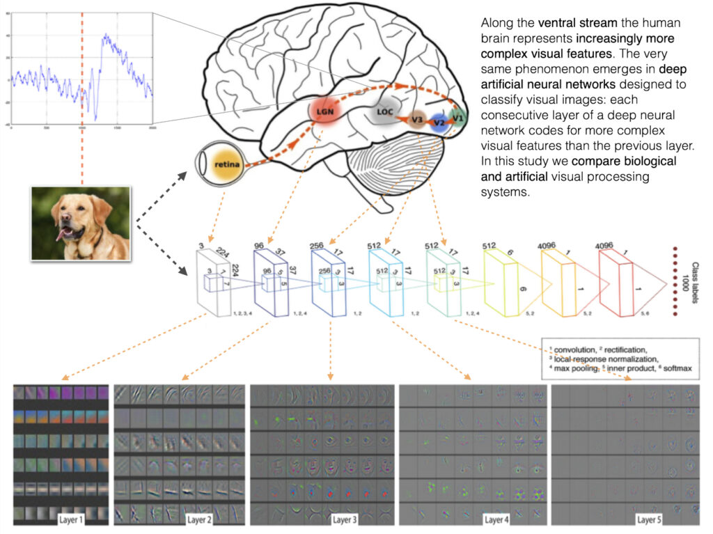
The attention that was given to this comparison is well-justified — the fact that the complexity of visual representations follows the hierarchy (the deeper into the system the more abstract are the concepts represented by the layers) in both systems, without being explicitly programmed (apart from the imposed hierarchical structure of the convolutional layers) to do so, is a non-trivial occurrence: two different systems evolved (biological via evolution, artificial via learning with optimisation) similar mechanisms for visual representations.

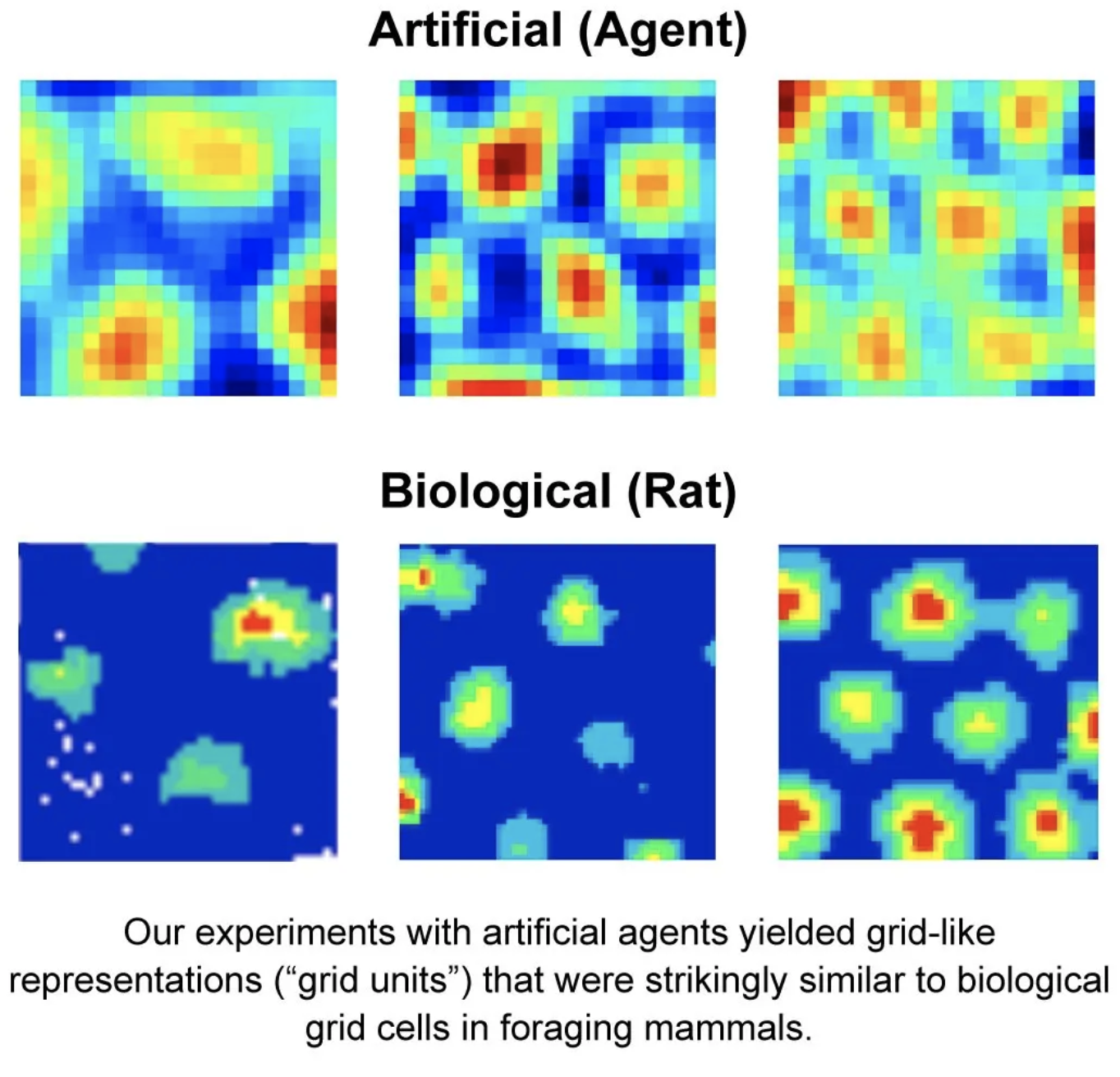
Representing spatial information in grids

In 2014, the Nobel Prize in Physiology or Medicine was awarded for the discovery of cells that constitute the positioning system in the brain (O’Keefe, 1976; Sargolini et al., 2006).

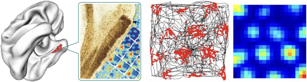
Banino et al. (2018) demonstrated that an artificial agent trained with reinforcement learning to navigate a maze starts to form periodic space representation similar to that provided by the grid cells. This representation “provided an effective basis for an agent to locate goals in challenging, un- familiar, and changeable environments”.

Successor representations

The trade-off between model-based and model-free methods is a long-standing question in reinforcement learning (RL), an area of machine learning that provides a framework to explore how an agent that is interacting with an environment can learn a behavior policy that maximizes a reward. As the name suggests, the model-based methods rely on the agent having access to the model of the environment, while model-free agents try to map observations directly onto actions or reward value estimates. While having a model would allow an agent to use it to plan ahead and be more sample efficient during learning, it also poses significant challenges as learning a model of the environment, especially if the environment is complex, is a very hard task on its own. Many successful results in RL were achieved with model-free methods as those are easier to implement and learning the mapping between the observations and the actions is in most cases sufficient and is easier than figuring out the full model of the environment.

The idea of successor representations (Dayan, 1993) lies in-between those two approaches. During the learning the agent counts how often the transition between a state \(s_a\) and state \(s_b\) has occurred. After interacting with the environment for some time the agent forms what is called an occupancy matrix M, which holds empirical evidence of transitioning between the states. This matrix is much easier to obtain than a full model of the environment and at the same time it provides some of the benefits of the model-based approach by allowing to model which transition is likely to occur next.

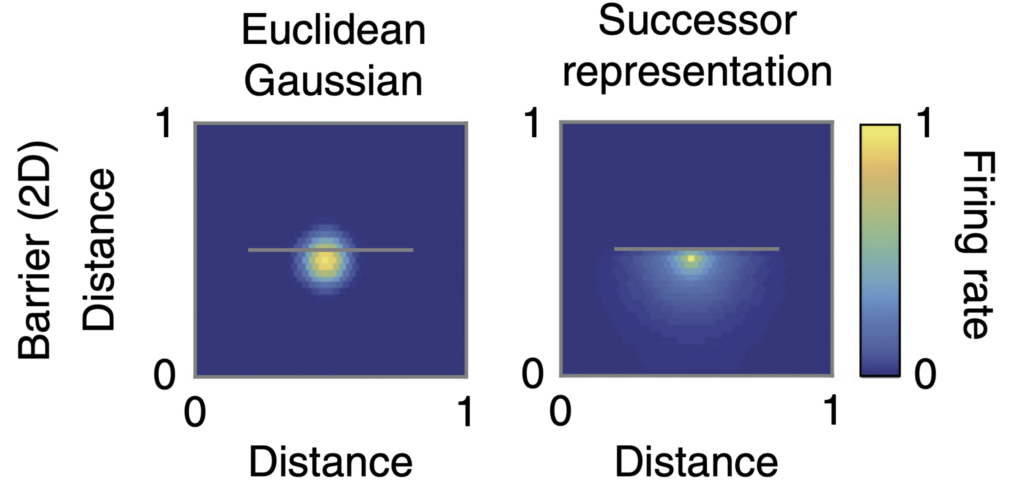
The hypothesis that the brain is using successor representations states that the brain is storing the occupancy probabilities of future states and is supported by behavioral (Tolman, 1948; Russek et al., 2017) and neural evidence (Alvernhe, Save, and Poucet, 2011; Stachenfeld, Botvinick, and Gershman, 2017). Using this statistic the brain can estimate which states are likely to occur next, serving as a computationally efficient approximation of a full-fledged environment model. The revival of the original concept in the context of RL (Momennejad et al., 2017) proposes a way to introduce some of the benefits of model-based methods without sacrificing the efficiency and ease of implementation of model-free methods.

Predictive coding and GANs

The theory of predictive coding (Rao and Ballard, 1999) proposes that the brain learns a statistical model of the sensory input and uses that model to predict neural responses to sensory stimuli. Only in the case when the prediction does not match the actual response the brain propagates the mismatch to the next level of the processing hierarchy. By building and memorizing an internal model of the sensory input such mechanism would reduce the redundancy of fully processing each sensory input anew at all levels and thus greatly reduce the processing load on the sensory system.

We find that this mechanism bears curious similarities to the mechanism used in Generative Adversarial Networks (GANs, Goodfellow et al., 2014). The purpose of the training process is to create a model called Generator that given a random (or preconditioned) input will generate a data sample (an image for example) that is indistinguishable from the distribution of data samples in the training data set. The learning process is guided by the second component of the system – a Discriminator, who’s job is to tell apart the real data samples from the ones generated by the Generator. If it call tell them apart, the Generator is not doing a good enough job and must improve.

To a young biological brain everything is novel and surprising. Brain’s predictive model (a “Generator” in this analogy) cannot predict what the sensory input will be like and the prediction error (“Discriminator’s” success) is high. Constant state of surprise, however, is quite taxing on the brain, so it must learn to ignore the inputs that are not important — train its “Generator” to lull the “Discriminator”, resulting in a system that only reacts to “out of distribution” samples in the environment.

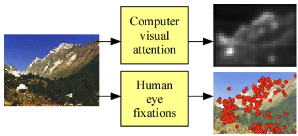
Visual attention

Our visual system does not process everything that is present in our field of view equally. Instead it focuses on some parts of the visual field at a time, which is demonstrated well by experiments exploring change blindness in humans. This general mechanism is what we call visual attention and it presents another curious similarity between biological and artificial mechanisms of vision — it turned out that implementing this idea approach in artificial systems of visual recognition leads to better efficiently and even higher object categorisation performance (Mnih 2014, Wang 2017, and other works).

Dopamine reward prediction and temporal difference learning

Deeper in your brain, below the cortex, where structures are evolutionary old and support basic functions there is an area called the basal ganglia. Among the nuclei comprising basal ganglia there are two that are of interest for this section of our overview, one is called ventral tegmental area (VTA) and the other substantia nigra. These two areas produce a neuromodulator molecule dopamine, that is involved in the feeling of pleasure, motivation, control of memory, mood, sleep, reward mechanisms, learning, concentration, movement and other body functions.

In 1997 W. Schultz, P. Dayan and P. R. Montague published a result linking the firing of dopaminergic neurons in those areas to error in animal’s prediction of whether it will get a reward (Schultz 1997).

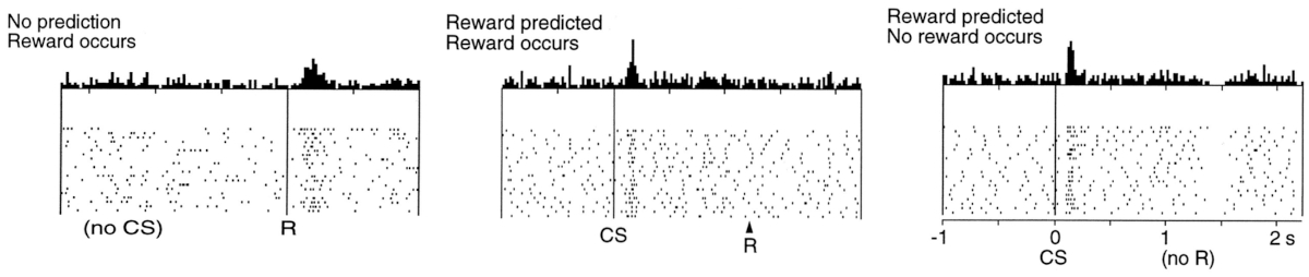
They demonstrated that the rate of firing of dopamine neurons closely matches reward prediction error in temporal difference (TD) learning algorithm. To appreciate how strong was the match between biology and an artificial algorithm that they have found we need to short explanation about the idea of what a reward prediction is in its formal representation.

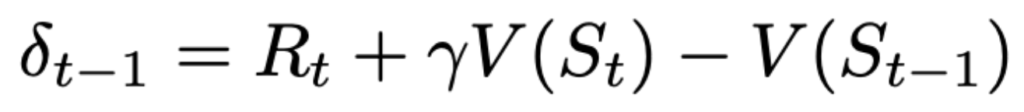
The prediction error that we make at time \(t-1\) about what reward we will get at time \(t\) consists of (a) \(R_t\) — the actual reward that was received at time \(t\) plus (b) our estimate of the reward from there on represented by \(V(S_t)\) adjusted by a discount factor \(\gamma\) that is conceptually unimportant right now. These two terms (a) and (b) are a sum of “what I got” and “what I am going to get from here on”. This is compared against my estimate that I had one time moment ago represented by the term (c) \(V(S_{t-1})\). So the difference between what I thought I will get and what I actually got one step later and from there on represents the prediction error, which is quite logical and intuitive.

The curious similarity between empirical observations of dopaminergic response and the way the TD error of a simple reinforcement learning algorithm is calculated is shown in the next image.

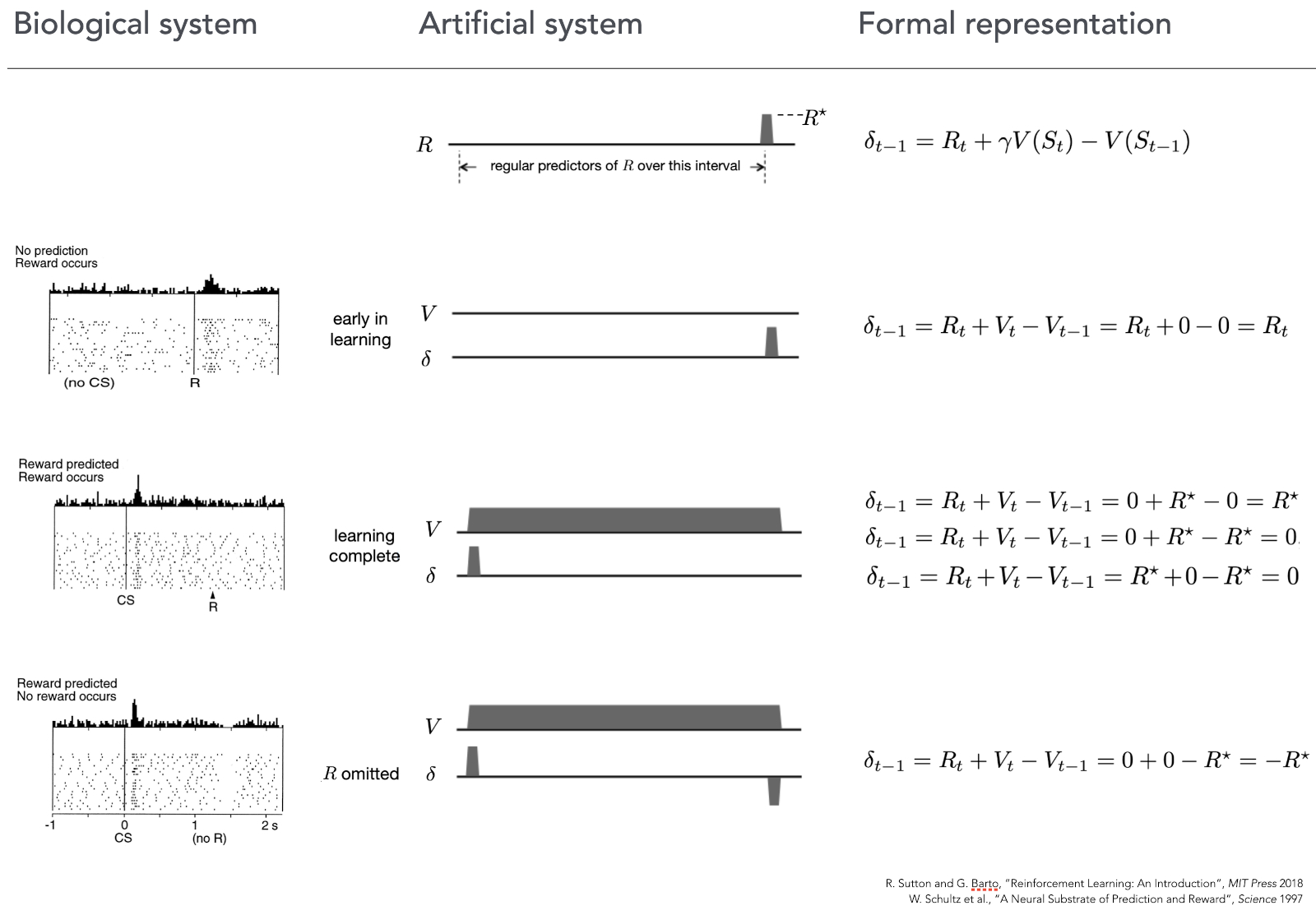
In the first row we can see the familiar equation on the right, and an artificial “experiment” in the middle, where a reward is given at the end of the trial (indicated by \(R*\)).

The second row presents the case when neither the biological (left) nor the artificial (middle) system can predict the reward, they are completely new to this situation and make not predictions. As we can see on the left image, in this situation like this, when a reward is given to an animal dopaminergic neurons start firing indicating a positive prediction error (they were not expecting anything, but suddenly there was a reward). Same can be seen in the artificial system (middle, right) the prediction \(V\) is flat (because the system has not learn anything yet and makes no predictions about the reward), and then, when at the end of the run it receives the reward the prediction error \(\sigma\) jumps up! Exactly the same reaction as the biological system had.

The third row of the image shows the case where both the animal, and the artificial system are trained to know that after a stimulus there will be a reward. Amazingly we can see that right after the presentation of the stimulus (CS) dopaminergic neurons fire as if there was a reward – they make a prediction that the reward will come. Notable when the reward actually comes (R) there is no activity – everything went “as expected”. The artificial counterpart in the middle shows that right from the beginning of the experiment the total reward estimation \(V\) is high up, so the prediction is made already at the start, same as was the case for the biological system. And when the reward comes, the expectation error \(\sigma\) is rightfully 0.

The final row shows what happens if we present the stimulus and make both systems to expect the reward, but then withhold it. Biological system predict right after the stimulus (CS) that there will be a reward, but now, at the moment when the reword should have appeared (R) it signals that the prediction was wrong, not in a negative way – and the activity of those neurons go down. This behavior is precisely followed by TD equation – omitting the reward at the end of the run causes \(\sigma\) to be \(-R\), signalling wrongfully optimistic prediction.

This match was a very strong indication that biological and artificial mechanisms of reinforcement learning have something in common and led to further investigations on comparing the formal mathematical framework of RL with neural circuitry of a mammalian brain, still an active area of scientific research.

Not only similarities: Backpropagation

The comparison on the level of algorithms and representation would not be complete without mentioning at least this one difference: the backpropagation algorithm, which is the main algorithm for training neural networks, is an unlikely candidate for how the brain solves the problem of synaptic credit assignment.

The training process of artificial neural networks consists of a very large number of small weight updates. Each connection between pairs of units in an ANN has a certain value (weight), when a input (like an image, represented as a matrix of numbers) is given to the network, the values of pixels are multiplied with the values on the corresponding connections (weights) and the results are sent to the next layer of the network. In this manner the initial input propagates through the whole network layer by layer until it reaches the final layer of the network. By reading out the values of the final layer we obtain the “answer” that the network thinks is the right one for the input we provided. For example if the task that a network is solving is image classification and we’ve given it an image of a cat as an input, then from the final layer we should read the pattern of activations that corresponds to the answer “cat”. If it does not — the backpropagation algorithms kicks in and traverses the whole network backwards, assigning blame to each particular connection for it’s contribution to the erroneous answer. The larger was the contribution of a particular weight, the higher the blame is assigned to it, and the larger change it will undergo during the upcoming update step to move its value closer to what it should have been in order for the whole network to provide that correct “cat” answer.

However due to a number of reasons reviewed in this presentation (Slide 6) by Geoffrey Hinton, this mathematic tool in not available to our brain, so they must be doing something else, or if similar, then at least only very local. We know that the brain retains knowledge by changing the strength of synaptic connections between neurons. Which means that there must a certain mechanism which will indicate how much each particular connection must be changed. But it looks like backpropagation is not that mechanism.

Conclusions about the level of algorithms and representations

In this lengthy section we went over multiple examples of how certain mechanisms and representations bear curious similarities in our brains and in machine learning algorithms. Some of them can be explained by something trivial, some other ones, however, evade simple explanations and allow us to think about the rules of computation that are being imposed by our physical reality.

The common goal of computation

On the computational level, the one that reflects the goal and purpose of the computation, biological and artificial systems are often identical: object and speech recognition, speech synthesis, decision-making based on observations, spatial orientation – these are some of the examples of computational goals that biological and artificial systems share. Those goals are given to the artificial systems by us, their creators, so it is no wonder that on this level we can easily find them very similar.

On the final note, perhaps this similarity and alignment of our goals and purposes is an argument in favour of the idea to attempt and connect mind and machine into a signal cognitive apparatus, something that for is mostly the in the realm of science fiction, but with the advances in neuroimaging tehcnologies and brain-computer interfaces, perhaps this field and technological direction will be gaining more and more traction.